29 BRIN

29.1 Overview

Unlike other indexes that are optimized to quickly find the required rows, BRIN¹ is designed to filter out unnecessary rows. This access method was created primarily for large tables of several terabytes and up, so a smaller index size takes priority over search accuracy.

To speed up search, the whole table is split into ranges, hence the name: Block Range Index. Each range comprises several pages. The index does not store TIDs, keeping only a summary on the data of each range. For ordinal data types, it is the minimal and the maximal values in the simplest case, but different operator classes may collect different information on values in a range.

The number of pages in a range is defined at the time of the index creation based on the value of the pages_per_range storage parameter. (default: 128)

If a query condition references an indexed column, all the ranges that are guaranteed to have no matches can be skipped. The pages of all the other ranges are returned by the index as a lossy bitmap; all the rows of these pages have to be rechecked. (p. 342)

Thus, BRIN works well for columns with localized values (that is, for columns in which values stored close to each other have similar summary information properties). For ordinal data types, it means that values must be stored in ascending or descending order, that is, have high correlation between their physical location and the logical order defined by the greater than and less than operations. For other types of summary information, “similar properties” may vary. (p. 284)

It will not be wrong to think of BRIN as an accelerator of sequential heap scans rather than an index in the conventional sense of the word. It can be regarded as an alternative to partitioning, with each range representing a virtual partition.

29.2 Example

Our demo database contains no tables that are large enough for BRIN, but we can imagine that analytical reports demand that we have a denormalized table containing summary information on all the departed and arrived flights of a particular airport, down to the occupied seats. The data for each airport is updated daily, as soon as it is midnight in the corresponding timezone. The added data is neither updated nor deleted.

The table looks as follows:

CREATE TABLE flights_bi(
  airport_code char(3),
  airport_coord point,         -- airport coordinates
  airport_utc_offset interval, -- timezone
  flight_no char(6),
  flight_type text,            -- departure or arrival
  scheduled_time timestamptz,
  actual_time timestamptz,
  aircraft_code char(3),
  seat_no varchar(4),
  fare_conditions varchar(10), -- travel class
  passenger_id varchar(20),
  passenger_name text
);

Data loading can be emulated using nested loops:² the outer loop will correspond to days (the demo database stores annual data), while the inner loop will be based on timezones. As a result, the loaded data will be more or less ordered at least by time and airports, even though it is not explicitly sorted within the loop.

I will load an existing copy of the database that takes roughly 4 GB and contains about 30 million rows:³

postgres$ pg_restore -d demo -c flights_bi.dump
=> ANALYZE flights_bi;
=> SELECT count(*) FROM flights_bi;
  count
----------
 30517076
(1 row)
=> SELECT pg_size_pretty(pg_total_relation_size('flights_bi'));
 pg_size_pretty
----------------
 4129 MB
(1 row)

We can hardly call it a large table, but this data volume will be enough to demonstrate how BRIN works. I will create an index in advance:

=> CREATE INDEX ON flights_bi USING brin(scheduled_time);
=> SELECT pg_size_pretty(pg_total_relation_size(
  'flights_bi_scheduled_time_idx'
));
 pg_size_pretty
----------------
 184 kB
(1 row)

It takes very little space with the default settings.

A B-tree index is a thousand times bigger, even if data deduplication is enabled. True, its efficiency is also much higher, but an additional volume can turn out to be unaffordable luxury for really large tables. (v. 13)

=> CREATE INDEX flights_bi_btree_idx ON flights_bi(scheduled_time);
=> SELECT pg_size_pretty(pg_total_relation_size(
  'flights_bi_btree_idx'
));
 pg_size_pretty
----------------
 210 MB
(1 row)
=> DROP INDEX flights_bi_btree_idx;

29.3 Page Layout

The zero page of a BRIN index is called the metapage; it keeps information on the index structure.

At a certain offset from the metadata, there are pages with summary information. Each index entry in such a page contains a summary of a particular block range.

The space between the metapage and the summary information is taken by the range map, which is sometimes also referred to as a reverse map (hence the common revmap abbreviation). It is effectively an array of pointers to the corresponding index rows; the index number in this array corresponds to the range number.

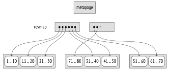
As the table is expanding, the size of the range map also grows. If the map does not fit the allotted pages, it overtakes the next page, and all the index entries previously located in this page are transferred to other pages. Since a page can accommodate many pointers, such transfers are quite rare.

BRIN index pages can be displayed by the pageinspect extension, as usual. The metadata includes the size of the range and the number of pages reserved for the range map:

=> SELECT pagesperrange, lastrevmappage
FROM brin_metapage_info(get_raw_page(
  'flights_bi_scheduled_time_idx', 0
));
 pagesperrange | lastrevmappage
---------------+----------------
           128 |              4
(1 row)

Here the range map takes four pages, from the first to the fourth one. We can take a look at the pointers to index entries containing summarized data:

=> SELECT *
FROM brin_revmap_data(get_raw_page(
  'flights_bi_scheduled_time_idx', 1
));
  pages
----------
 (6,197)
 (6,198)
 (6,199)
 ...
 (6,195)
 (6,196)
(1360 rows)

If the range is not summarized yet, the pointer in the range map is NULL.

And here are the summaries for several ranges:

=> SELECT itemoffset, blknum, value
FROM brin_page_items(
  get_raw_page('flights_bi_scheduled_time_idx', 6),
  'flights_bi_scheduled_time_idx'
)
ORDER BY blknum
LIMIT 3 \gx
-[ RECORD 1 ]--------------------------------------------------
itemoffset | 197
blknum     | 0
value      | {2016-08-15 02:45:00+03 .. 2016-08-15 16:20:00+03}
-[ RECORD 2 ]--------------------------------------------------
itemoffset | 198
blknum     | 128
value      | {2016-08-15 05:50:00+03 .. 2016-08-15 18:55:00+03}
-[ RECORD 3 ]--------------------------------------------------
itemoffset | 199
blknum     | 256
value      | {2016-08-15 07:15:00+03 .. 2016-08-15 18:50:00+03}
-[ RECORD 4 ]--------------------------------------------------
itemoffset | 200
blknum     | 384
value      | 2016-08-15 07:55:00+03 .. 2016-08-15 20:20:00+03

29.4 Search

If a query condition is supported by the BRIN index,⁴ the executor scans the range map and the summary information for each range. If the data in a range may match the search key, all the pages that belong to this range are added to the bitmap. Since BRIN does not keep IDs of separate tuples, the bitmap is always lossy.

Matching the data against the search key is performed by the consistency function, which interprets range summary information. Non-summarized ranges are always added to the bitmap.

The received bitmap is used to scan the table in the usual manner. It is important to mention that heap page reads happen sequentially, block range by block range, and prefetching is employed. (p. 340)

29.5 Summary Information Updates

Value Insertion

As a new tuple is added into a heap page, the summary information in the corresponding index range gets updated.⁵ The range number is calculated based on the page number using simple arithmetic operations, and the summary information is then located by the range map.

To determine whether the current summary information has to be expanded, the addition function is employed. If an expansion is required and the page has enough free space, it is done in-place (without adding a new index entry).

Suppose we have added a tuple with value 42 to page 13. The range number is calculated by integer division of page number by the size of the range. Assuming that the range size equals four pages, we get range number 3; since range numbering is zero-based, we take the fourth pointer in the range map. The minimal value in this range is 31, the maximal one is 40. The added value falls outside these limits, so the maximal value is increased:

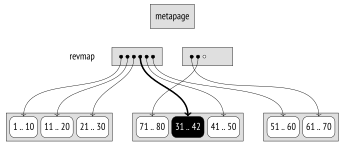
If an in-place update is impossible, a new entry is added, and the range map is modified.

Range Summarization

Everything said above applies to scenarios when a new tuple appears in an already summarized range. When an index is being built, all the existing ranges are summarized, but as the table grows, new pages may fall outside these ranges.

If an index is created with the autosummarize storage parameter enabled, the new range will be summarized at once. But in data warehouses, where rows are usually added in large batches rather than one by one, this mode can seriously slow down insertion. (default: off)

By default, new ranges are not summarized right away. It does not affect index correctness because ranges with no summary information are always scanned. Summarization is performed asynchronously, either during table vacuuming or when initiated manually by calling the brin_summarize_new_values function (or the brin_summarize_range function that processes a single range). (p. 112)

Range summarization⁶ does not lock the table for updates. At the beginning of this process, a placeholder entry is inserted into the index for this range. If the data in the range is changed while this range is being scanned, the placeholder will be updated with the summary information on these changes. Then the union function will unite this data with the summary information on the corresponding range.

In theory, summary information could sometimes shrink after some rows are deleted. But while GiST indexes can redistribute data after a page split, summary information of BRIN indexes never shrinks and can only get wider. Shrinking is usually not required here because a data storage is typically used only for appending new data. You can manually delete summary information by calling the brin_desummarize_range function for this range to be summarized again, but there is no clue as to which ranges might benefit from it. (p. 445)

Thus, BRIN is primarily targeted at tables of very large size, which either have minimal updates that add new rows mostly to the end of the file, or are not updated at all. It is mainly used in data warehouses for building analytical reports.

29.6 Minmax Classes

For data types that allow comparing values, summary information includes at least the maximal and minimal values. The corresponding operator classes contain the word minmax in their names:⁷

=> SELECT opcname
FROM pg_am am
  JOIN pg_opclass opc ON opcmethod = am.oid
WHERE amname = 'brin'
AND opcname LIKE '%minmax_ops'
ORDER BY opcname;
        opcname
------------------------
 bit_minmax_ops
 bpchar_minmax_ops
 bytea_minmax_ops
 ...
 timetz_minmax_ops
 uuid_minmax_ops
 varbit_minmax_ops
(26 rows)

Here are the support functions of these operator classes:

=> SELECT amprocnum, amproc::regproc
FROM pg_am am
  JOIN pg_opclass opc ON opcmethod = am.oid
  JOIN pg_amproc amop ON amprocfamily = opcfamily
WHERE amname = 'brin'
AND opcname = 'numeric_minmax_ops'
ORDER BY amprocnum;
 amprocnum |         amproc
-----------+------------------------
         1 | brin_minmax_opcinfo
         2 | brin_minmax_add_value
         3 | brin_minmax_consistent
         4 | brin_minmax_union
(4 rows)

The first function returns the operator class metadata, and all the other functions have already been described: they insert new values, check consistency, and perform union operations.

The minmax class includes the same comparison operators that we have seen for B-trees: (p. 432)

=> SELECT amopopr::regoperator, oprcode::regproc, amopstrategy
FROM pg_am am
  JOIN pg_opclass opc ON opcmethod = am.oid
  JOIN pg_amop amop ON amopfamily = opcfamily
  JOIN pg_operator opr ON opr.oid = amopopr
WHERE amname = 'brin'
AND opcname = 'numeric_minmax_ops'
ORDER BY amopstrategy;
       amopopr       |  oprcode   | amopstrategy
---------------------+------------+--------------
 <(numeric,numeric)  | numeric_lt |            1
 <=(numeric,numeric) | numeric_le |            2
 =(numeric,numeric)  | numeric_eq |            3
 >=(numeric,numeric) | numeric_ge |            4
 >(numeric,numeric)  | numeric_gt |            5
(5 rows)

Choosing Columns to be Indexed

Which columns does it make sense to index using this operator class? As mentioned earlier, such indexes work well if the physical location of rows correlates with the logical order of values.

Let’s check it for the above example.

=> SELECT attname, correlation, n_distinct
FROM pg_stats
WHERE tablename = 'flights_bi'
ORDER BY correlation DESC NULLS LAST;
      attname       |  correlation   |  n_distinct
--------------------+----------------+--------------
 scheduled_time     |      0.9999949 |        25926
 actual_time        |      0.9999948 |        34469
 fare_conditions    |      0.7976897 |            3
 flight_type        |      0.4981733 |            2
 airport_utc_offset |      0.4440067 |           11
 aircraft_code      |     0.19249801 |            8
 airport_code       |    0.061483838 |          104
 seat_no            |   0.0024594965 |          461
 flight_no          |   0.0020146023 |          710
 passenger_id       | -0.00046121294 | 2.610987e+06
 passenger_name     |   -0.012388787 |         8618
 airport_coord      |                |            0
(12 rows)

The data is ordered by time (both scheduled and actual time; there is little difference, if any): new entries are added in chronological order, and as the data is neither updated nor deleted, all the rows get into the main fork of the table sequentially, one after another. (p. 25)

Columns fare_conditions, flight_type, and airport_utc_offset have relatively high correlation, but they store too few distinct values.

The correlation in other columns is too low for their indexing with the minmax operator class to be of any interest.

Range Size and Search Efficiency

An appropriate range size can be determined based on the number of pages used to store particular values.

Let’s take a look at the scheduled_time column and get the information on all the flights performed in 24 hours. We first have to find out how many table pages are taken by the data related to this time interval.

To get this number, we can use the fact that a TID consists of a page number and an offset. Unfortunately, there is no built-in function to break down a TID into these two components, so we will have to write our own clumsy function to perform type casting via a text representation:

=> CREATE FUNCTION tid2page(t tid) RETURNS integer
LANGUAGE sql
RETURN (t::text::point)[0]::integer;

Now we can see how days are distributed through the table:

=> SELECT min(numblk), round(avg(numblk)) avg, max(numblk)
FROM (
  SELECT count(distinct tid2page(ctid)) numblk
  FROM flights_bi
  GROUP BY scheduled_time::date
) t;
 min  | avg  | max
------+------+------
 1192 | 1447 | 1512
(1 row)

As we can notice, the data distribution is not quite uniform. With a standard range size of 128 pages, each day will take from 9 to 12 ranges. While fetching the data for a particular day, the index scan will return both the rows that are really needed and some rows related to other days that got into the same ranges. The bigger the range size, the more extra boundary values will be read; we can change their number by reducing or increasing the range size.

Let’s try out a query for some particular day (I have already created an index with the default settings). For simplicity, I will forbid parallel execution:

=> SET max_parallel_workers_per_gather = 0;
=> \set d '2016-08-15 02:45:00+03'
=> EXPLAIN (analyze, buffers, costs off, timing off, summary off)
SELECT * FROM flights_bi
WHERE scheduled_time >= :'d'::timestamptz
  AND scheduled_time < :'d'::timestamptz + interval '1 day';
                             QUERY PLAN
---------------------------------------------------------------------
 Bitmap Heap Scan on flights_bi (actual rows=81964 loops=1)
   Recheck Cond: ((scheduled_time >= '2016-08-15 02:45:00+03'::ti...
   Rows Removed by Index Recheck: 11606
   Heap Blocks: lossy=1536
   Buffers: shared hit=1561
   -> Bitmap Index Scan on flights_bi_scheduled_time_idx
       (actual rows=15360 loops=1)
       Index Cond: ((scheduled_time >= '2016-08-15 02:45:00+03'::...
       Buffers: shared hit=25
 Planning:
   Buffers: shared hit=1
(11 rows)

We can define an efficiency factor of a BRIN index for a particular query as a ratio between the number of pages skipped in an index scan and the total number of pages in the table. If the efficiency factor is zero, the index access degrades to sequential scanning (without taking overhead costs into account). The higher the efficiency factor, the fewer pages have to be read. But as some pages contain the data to be returned and cannot be skipped, the efficiency factor is always smaller than one. (p. 348)

In this particular case, the efficiency factor is $\frac{528417-1561}{528417}$ ≈ 0.997, where 528,417 is the number of pages in the table.

However, we cannot draw any meaningful conclusions based on a single value. Even if we had uniform data and ideal correlation, the efficiency would still vary because, at the very least, range boundaries will not match page boundaries. We can get the full picture only if we treat the efficiency factor as a random value and analyze its distribution.

For our example, we can select all the different days of the year, check the execution plan for each value, and calculate statistics based on this selection. We can easily automate this process because the EXPLAIN command can return the results in the JSON format, which is convenient to parse. I will not provide all the code here, but the following snippet contains all the important details:

=> DO $$
DECLARE
  plan jsonb;
BEGIN
  EXECUTE
    'EXPLAIN (analyze, buffers, timing off, costs off, format json)
     SELECT * FROM flights_bi
     WHERE scheduled_time >= $1
       AND scheduled_time < $1 + interval ''1 day'''
  USING '2016-08-15 02:45:00+03'::timestamptz
  INTO plan;
  RAISE NOTICE 'shared hit=%, read=%',
    plan -> 0 -> 'Plan' ->> 'Shared Hit Blocks',
    plan -> 0 -> 'Plan' ->> 'Shared Read Blocks';
END;
$$;
NOTICE:  shared hit=1561, read=0
DO

The results can be visually displayed as a box plot, also known as a “box-and-whiskers.” The whiskers here denote the first and fourth quartiles (that is, the right whisker gets 25 % of the largest values, while the left one gets 25 % of the smallest values). The box itself holds the remaining 50 % of values and has the median value marked. What is more important, this compact representation enables us to visually compare different results. The following illustration shows the efficiency factor distribution for the default range size and for two other sizes that are four times larger and smaller.

As we could have expected, the search accuracy and efficiency are high even for rather large ranges.

The dashed line here marks the average value of the maximal efficiency factor possible for this query, assuming that one day takes roughly $\frac{1}{365}$ of the table.

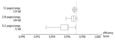
Note that the rise in efficiency comes at the expense of the index size increase. BRIN is quite flexible in letting you find the balance between the two.

Properties

BRIN properties are hardwired and do not depend on operator classes.

Access Method Properties

=> SELECT a.amname, p.name, pg_indexam_has_property(a.oid, p.name)
FROM pg_am a, unnest(array[
  'can_order', 'can_unique', 'can_multi_col',
  'can_exclude', 'can_include'
]) p(name)
WHERE a.amname = 'brin';
 amname |     name      | pg_indexam_has_property
--------+---------------+-------------------------
 brin   | can_order     | f
 brin   | can_unique    | f
 brin   | can_multi_col | t
 brin   | can_exclude   | f
 brin   | can_include   | f
(5 rows)

Obviously, neither sorting nor uniqueness properties are supported. Since a BRIN index always returns a bitmap, exclusion constraints are not supported either. Neither do additional INCLUDE columns make any sense, as even indexing keys are not stored in BRIN indexes.

However, we can create a multicolumn BRIN index. In this case, summary information for each column is collected and stored in a separate index entry, but they still have a common range mapping. Such an index is useful if the same range size is applicable to all the indexed columns.

Alternatively, we can create separate BRIN indexes for several columns and take advantage of the fact that bitmaps can be merged together. For example: (p. 343)

=> CREATE INDEX ON flights_bi USING brin(airport_utc_offset);
=> EXPLAIN (analyze, costs off, timing off, summary off)
SELECT *
FROM flights_bi
WHERE scheduled_time >= :'d'::timestamptz
  AND scheduled_time < :'d'::timestamptz + interval '1 day'
  AND airport_utc_offset = '08:00:00';
                             QUERY PLAN
---------------------------------------------------------------------
 Bitmap Heap Scan on flights_bi (actual rows=1658 loops=1)
   Recheck Cond: ((scheduled_time >= '2016-08-15 02:45:00+03'::ti...
   Rows Removed by Index Recheck: 14077
   Heap Blocks: lossy=256
   -> BitmapAnd (actual rows=0 loops=1)
       -> Bitmap Index Scan on flights_bi_scheduled_time_idx (act...
           Index Cond: ((scheduled_time >= '2016-08-15 02:45:00+0...
       -> Bitmap Index Scan on flights_bi_airport_utc_offset_idx ...
           Index Cond: (airport_utc_offset = '08:00:00'::interval)
(9 rows)

Index-Level Properties

=> SELECT p.name, pg_index_has_property(
  'flights_bi_scheduled_time_idx', p.name
)
FROM unnest(array[
  'clusterable', 'index_scan', 'bitmap_scan', 'backward_scan'
]) p(name);
     name      | pg_index_has_property
---------------+-----------------------
 clusterable   | f
 index_scan    | f
 bitmap_scan   | t
 backward_scan | f
(4 rows)

Obviously, bitmap scanning is the only supported access type.

Lack of clusterization may seem puzzling. Since BRIN is sensitive to the physical order of rows, it is quite logical to assume that it should support reordering, which would maximize its efficiency. But clusterization of large tables is anyway a luxury, taking into account all the processing and extra disk space required to rebuild a table. Besides, as the example of the flights_bi table shows, some ordering in data storages can occur naturally.

Column-Level Properties

=> SELECT p.name, pg_index_column_has_property(
  'flights_bi_scheduled_time_idx', 1, p.name
)
FROM unnest(array[
  'orderable', 'distance_orderable', 'returnable',
  'search_array', 'search_nulls'
]) p(name);
        name        | pg_index_column_has_property
--------------------+------------------------------
 orderable          | f
 distance_orderable | f
 returnable         | f
 search_array       | f
 search_nulls       | t
(5 rows)

The only available column-level property is NULL support. To track NULL values in a range, summary information provides a separate attribute:

=> SELECT hasnulls, allnulls, value
FROM brin_page_items(
  get_raw_page('flights_bi_airport_utc_offset_idx', 6),
  'flights_bi_airport_utc_offset_idx'
)
WHERE itemoffset= 1;
 hasnulls | allnulls |         value
----------+----------+------------------------
 f        | f        | {03:00:00 .. 03:00:00}
(1 row)

29.7 Minmax-Multi Classes

The established correlation can be easily disrupted by data updates. The reason is not an actual modification of a particular value but rather the MVCC design itself: an old version of a row may be deleted in one page, while its new version may be inserted into any location that is currently free, so the original row order cannot be preserved. (v. 14) (p. 66)

To minimize this effect to some extent, we can reduce the value of the fillfactor storage parameter to leave more space in the page for future updates. But is it really worth increasing the size of an already huge table? Besides, deletions will anyway free some space in existing pages, thus preparing traps for new tuples that would otherwise get to the end of the file.

Such a situation can be easily emulated. Let’s delete 0.1 % of randomly chosen rows and vacuum the table to clean up some space for new tuples:

=> WITH t AS (
  SELECT ctid
  FROM flights_bi TABLESAMPLE BERNOULLI(0.1) REPEATABLE(0)
)
DELETE FROM flights_bi
WHERE ctid IN (SELECT ctid FROM t);
DELETE 30180
=> VACUUM flights_bi;

Now let’s add some data for a new day in one of the timezones. I will simply copy the data of the previous day:

=> INSERT INTO flights_bi
SELECT airport_code, airport_coord, airport_utc_offset,
  flight_no, flight_type, scheduled_time + interval '1 day',
  actual_time + interval '1 day', aircraft_code, seat_no,
 fare_conditions, passenger_id, passenger_name
FROM flights_bi
WHERE date_trunc('day', scheduled_time) = '2017-08-15'
  AND airport_utc_offset = '03:00:00';
INSERT 0 40532

The performed deletion was enough to free some space in all or almost all the ranges. Getting into pages located somewhere in the middle of the file, new tuples have automatically expanded the ranges. For example, the summary information related to the first range used to cover less than a day, but now it comprises the whole year:

=> SELECT value
FROM brin_page_items(
  get_raw_page('flights_bi_scheduled_time_idx', 6),
  'flights_bi_scheduled_time_idx'
)
WHERE blknum = 0;
                       value
----------------------------------------------------
 {2016-08-15 02:45:00+03 .. 2017-08-16 09:35:00+03}
(1 row)

The smaller the date specified in the query, the more ranges have to be scanned. The graph shows the magnitude of the disaster:

To address this issue, we have to make the summary information a bit more sophisticated: instead of a single continuous range, we have to store several smaller ones that cover all the values when taken together. Then one of the ranges can cover the main set of data, while the rest will handle occasional outliers.

Such functionality is provided by minmax-multi operator classes:⁸

=> SELECT opcname
FROM pg_am am
  JOIN pg_opclass opc ON opcmethod = am.oid
WHERE amname = 'brin'
AND opcname LIKE '%minmax_multi_ops'
ORDER BY opcname;
           opcname
------------------------------
 date_minmax_multi_ops
 float4_minmax_multi_ops
 float8_minmax_multi_ops
 inet_minmax_multi_ops
 ...
 time_minmax_multi_ops
 timestamp_minmax_multi_ops
 timestamptz_minmax_multi_ops
 timetz_minmax_multi_ops
 uuid_minmax_multi_ops
(19 rows)

As compared to minmax operator classes, minmax-multi classes have one more support function that computes the distance between values; it is used to determine the range length, which the operator class strives to reduce:

=> SELECT amprocnum, amproc::regproc
FROM pg_am am
  JOIN pg_opclass opc ON opcmethod = am.oid
  JOIN pg_amproc amop ON amprocfamily = opcfamily
WHERE amname = 'brin'
AND opcname = 'numeric_minmax_multi_ops'
ORDER BY amprocnum;
 amprocnum |               amproc
-----------+------------------------------------
         1 | brin_minmax_multi_opcinfo
         2 | brin_minmax_multi_add_value
         3 | brin_minmax_multi_consistent
         4 | brin_minmax_multi_union
         5 | brin_minmax_multi_options
        11 | brin_minmax_multi_distance_numeric
(6 rows)

The operators of such classes are absolutely the same as those of the minmax classes.

Minmax-multi classes can take the values_per_range parameter, which defines the maximal allowed number of summarized values per range. A summarized value is represented by two numbers (an interval),while a separate point requires just one. If there are not enough values, some of the intervals are reduced.⁹ (default: 32)

Let’s build a minmax-multi index instead of the existing one. We will limit the number of allowed values per range to 16:

=> DROP INDEX flights_bi_scheduled_time_idx;
=> CREATE INDEX ON flights_bi USING brin(
  scheduled_time timestamptz_minmax_multi_ops(
    values_per_range = 16
  )
);

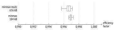
The graph shows that the new index brings the efficiency back to the original level. Quite expectedly, it leads to an increase in the index size:

29.8 Inclusion Classes

The difference between minmax and inclusion operator classes is roughly the same as the difference between B-trees and GiST indexes: the latter are designed for data types that do not support comparison operations, although mutual alignment of values still makes sense for them. Summary information for a particular range provided by inclusion operator classes is represented by the bounding box of the values in this range.

Here are these operator classes; they are not numerous:

=> SELECT opcname
FROM pg_am am
  JOIN pg_opclass opc ON opcmethod = am.oid
WHERE amname = 'brin'
AND opcname LIKE '%inclusion_ops'
ORDER BY opcname;
       opcname
---------------------
 box_inclusion_ops
 inet_inclusion_ops
 range_inclusion_ops
(3 rows)

The list of support functions is extended by one more mandatory function that merges two values, and by a bunch of optional ones:

=> SELECT amprocnum, amproc::regproc
FROM pg_am am
  JOIN pg_opclass opc ON opcmethod = am.oid
  JOIN pg_amproc amop ON amprocfamily = opcfamily
WHERE amname = 'brin'
AND opcname = 'box_inclusion_ops'
ORDER BY amprocnum;
 amprocnum |          amproc
-----------+---------------------------
         1 | brin_inclusion_opcinfo
         2 | brin_inclusion_add_value
         3 | brin_inclusion_consistent
         4 | brin_inclusion_union
        11 | bound_box
        13 | box_contain
(6 rows)

When dealing with values that can be compared, we relied on their correlation; but for other data types, no such statistic is collected,¹⁰ so it is hard to predict the efficiency of an inclusion-based BRIN index.

What is worse, correlation greatly affects cost estimation of an index scan. If such statistic is unavailable, it is taken as zero.¹¹ Thus, the planner has no way to tell between exact and fuzzy inclusion indexes, so it typically avoids using them altogether. (v. 3.1.1)

In this particular case, we can presume that it makes sense to build an index over airport coordinates, as longitude must correlate with the timezone.

Unlike GiST predicates, BRIN summary information has the same type as the indexed data; therefore, it is not so easy to build an index for points. But we can create an expression index by converting points into dummy rectangles:

=> CREATE INDEX ON flights_bi USING brin(box(airport_coord))
WITH (pages_per_range = 8);
=> SELECT pg_size_pretty(pg_total_relation_size(
  'flights_bi_box_idx'
));
 pg_size_pretty
----------------
 3816 kB
(1 row)

An index built over timezones with the same range size takes approximately the same volume (3288 kB).

The operators included into this class are similar to GiST operators. For example, a BRIN index can be used to speed up search for points in a certain area:

=> SELECT airport_code, airport_name
FROM airports
WHERE box(coordinates) <@ box '135,45,140,50';
 airport_code |      airport_name
--------------+-------------------------
 KHV          | Khabarovsk-Novy Airport
(1 row)

But as mentioned earlier, the planner refuses to use an index scan unless we turn off sequential scanning:

=> EXPLAIN (costs off)
SELECT *
FROM flights_bi
WHERE box(airport_coord) <@ box '135,45,140,50';
                         QUERY PLAN
------------------------------------------------------------
 Seq Scan on flights_bi
   Filter: (box(airport_coord) <@ '(140,50),(135,45)'::box)
(2 rows)
=> SET enable_seqscan = off;
=> EXPLAIN (analyze, costs off, timing off, summary off)
SELECT *
FROM flights_bi
WHERE box(airport_coord) <@ box '135,45,140,50';
                             QUERY PLAN
---------------------------------------------------------------------
 Bitmap Heap Scan on flights_bi (actual rows=511414 loops=1)
   Recheck Cond: (box(airport_coord) <@ '(140,50),(135,45)'::box)
   Rows Removed by Index Recheck: 630756
   Heap Blocks: lossy=19656
   -> Bitmap Index Scan on flights_bi_box_idx (actual rows=196560...
       Index Cond: (box(airport_coord) <@ '(140,50),(135,45)'::box)
(6 rows)
=> RESET enable_seqscan;

29.9 Bloom Classes

Operator classes based on the Bloom filter enable BRIN usage for any data types that support the equal to operation and have a hash function defined. They can also be applied to regular ordinal types if values are localized in separate ranges but their physical location has no correlation with the logical order. (v. 14)

The names of such operator classes contain the word bloom:¹²

=> SELECT opcname
FROM pg_am am
  JOIN pg_opclass opc ON opcmethod = am.oid
WHERE amname = 'brin'
AND opcname LIKE '%bloom_ops'
ORDER BY opcname;
        opcname
-----------------------
 bpchar_bloom_ops
 bytea_bloom_ops
 char_bloom_ops
 ...
 timestamptz_bloom_ops
 timetz_bloom_ops
 uuid_bloom_ops
(24 rows)

The classic Bloom filter is a data structure that enables you to quickly check whether an element belongs to a set. This filter is very compact, but it allows false positives: a set may be assumed to contain more elements than it actually does. But what is more important, false negatives are ruled out: the filter cannot decide that an element is not present in the set if it is actually there.

The filter is an array of m bits (also called a signature), which is originally filled with zeros. We select k different hash functions to map any element of the set to k bits of the signature. When an element is added to the set, each of the bits in the signature is set to one. Consequently, if all the bits that correspond to an element are set to one, the element may be present in the set; if there is at least one zero bit, the element is guaranteed to be absent.

In the case of BRIN indexes, the filter processes a set of values of an indexed column that belong to a particular range; the summary information for this range is represented by the built Bloom filter.

The accuracy of the Bloom filter depends on the signature length. In theoretical terms, the optimal number of signature bits can be estimated at m = $-\frac{n\log_2 p}{\ln 2}$, where n is the number of elements in the set and p is the probability of false positives.

These two settings can be adjusted using the corresponding operator class parameters:

• n_distinct_per_range defines the number of elements in a set; in this case, it is the number of distinct values in one range of an indexed column. This parameter value is interpreted just like statistics on distinct values: negative values indicate the fraction of rows in the range, not their absolute number. (default: -0.1) (p. 276)

• false_positive_rate defines the probability of false positives. (default: 0.01)

A near-zero value means that an index scan will almost certainly skip the ranges that have no searched values. But it does not guarantee exact search, as the scanned ranges will also contain extra rows that do not match the query. Such behavior is due to range width and physical data location rather than to the actual filter properties.

The list of support functions is extended by a hash function:

=> SELECT amprocnum, amproc::regproc
FROM pg_am am
  JOIN pg_opclass opc ON opcmethod = am.oid
  JOIN pg_amproc amop ON amprocfamily = opcfamily
WHERE amname = 'brin'
AND opcname = 'numeric_bloom_ops'
ORDER BY amprocnum;
 amprocnum |        amproc
-----------+-----------------------
         1 | brin_bloom_opcinfo
         2 | brin_bloom_add_value
         3 | brin_bloom_consistent
         4 | brin_bloom_union
         5 | brin_bloom_options
        11 | hash_numeric
(6 rows)

Since the Bloom filter is based on hashing, only the equality operator is supported:

=> SELECT amopopr::regoperator, oprcode::regproc, amopstrategy
FROM pg_am am
  JOIN pg_opclass opc ON opcmethod = am.oid
  JOIN pg_amop amop ON amopfamily = opcfamily
  JOIN pg_operator opr ON opr.oid = amopopr
WHERE amname = 'brin'
AND opcname = 'numeric_bloom_ops'
ORDER BY amopstrategy;
      amopopr       |  oprcode   | amopstrategy
--------------------+------------+--------------
 =(numeric,numeric) | numeric_eq |            1
(1 row)

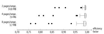
Let’s take the flight_no column that stores flight numbers; it has near-zero correlation, so it is useless for a regular range operator class. We will keep the default false-positive setting; as for the number of distinct values in a range, it can be easily calculated. For example, for an eight-page range we will get the following value:

=> SELECT max(nd)
FROM (
  SELECT count(distinct flight_no) nd
  FROM flights_bi
  GROUP BY tid2page(ctid) / 8
) t;
 max
-----
  22
(1 row)

For smaller ranges, this number will be even lower (but in any case, the operator class does not allow values smaller than 16).

We just have to create an index and check the execution plan:

=> CREATE INDEX ON flights_bi USING brin(
  flight_no bpchar_bloom_ops(n_distinct_per_range = 22)
)
WITH (pages_per_range = 8);
=> EXPLAIN (analyze, costs off, timing off, summary off)
SELECT *
FROM flights_bi
WHERE flight_no = 'PG0001';
                             QUERY PLAN
---------------------------------------------------------------------
 Bitmap Heap Scan on flights_bi (actual rows=5192 loops=1)
   Recheck Cond: (flight_no = 'PG0001'::bpchar)
   Rows Removed by Index Recheck: 122894
   Heap Blocks: lossy=2168
   -> Bitmap Index Scan on flights_bi_flight_no_idx (actual rows=...
       Index Cond: (flight_no = 'PG0001'::bpchar)
(6 rows)
=> RESET max_parallel_workers_per_gather;

The graph shows that for some flight numbers (represented by separate points that do not belong to any whiskers) the index does not work very well, but its overall efficiency is quite high: