23 Sorting and Merging
PostgreSQL 14 · Translated from Russian by Liudmila Mantrova · Chinese translation by Xiong Cancan
23.1 Merge Joins
A merge join processes data sets sorted by the join key and returns the result that is sorted in a similar way. Input sets may come pre-sorted following an index scan; otherwise, the executor has to sort them before the actual merge begins.1
Merging Sorted Sets
Let’s take a look at an example of a merge join; it is represented in the execution plan by the Merge Join node:2
The optimizer prefers this join method because it returns a sorted result, as defined by the ORDER BY clause. When choosing a plan, the optimizer notes the sort order of the data sets and does not perform any sorting unless it is really required. For example, if the data set produced by a merge join already has an appropriate sort order, it can be used in the subsequent merge join as is:
The first tables to be joined are ticket_flights and boarding_passes; both of them have a composite primary key (ticket_no, flight_id), and the result is sorted by these two columns. The produced set of rows is then joined with the tickets table, which is sorted by the ticket_no column.
The join requires only one pass over both data sets and does not take any additional memory. It uses two pointers to the current rows (which are originally the first ones) of the inner and outer sets.
If the keys of the current rows do not match, one of the pointers (that references the row with the smaller key) is going to be advanced to the next row until it finds a match. The joined rows are returned to the upper node, and the pointer of the inner set is advanced by one place. The operation continues until one of the sets is over.
This algorithm copes with duplicates of the inner set, but the outer set can contain them too. To address this issue, the algorithm has to be improved: if the key remains the same after the outer pointer is advanced, the inner pointer gets back to the first matching row. Thus, each row of the outer set will be matched to all the rows of the inner set with the same key.3
For the outer join, the algorithm is further tweaked a bit, but it is still based on the same principle.
Merge join conditions can use only the equality operator, which means that only equi-joins are supported (although support for other condition types is currently being implemented as well).4
Cost estimation. Let’s take a closer look at the previous example:
The startup cost of the join includes at least the startup costs of all the child nodes.
In general, it may be required to scan some fraction of the outer or inner set before the first match is found. It is possible to estimate this fraction by comparing (based on the histogram) the smallest join keys in the two sets.5 But in this particular case, the range of ticket numbers is the same in both tables. (p. 279)
The total cost comprises the cost of fetching the data from the child nodes and the computation cost.
Since the join algorithm stops as soon as one of the sets is over (unless the outer join is performed, of course), the other set may be scanned only partially. To estimate the size of the scanned part, we can compare the maximal key values in the two sets. In this example, both sets will be read in full, so the total cost of the join includes the sum of the total costs of both child nodes.
Moreover, if there are any duplicates, some of the rows of the inner set may be scanned several times. The estimated number of repeat scans equals the difference between the cardinalities of the join result and the inner set.6 In this query, these cardinalities are the same, which means that the sets contain no duplicates.
The algorithm compares join keys of the two sets. The cost of one comparison is estimated at the cpu_operator_cost value, while the estimated number of comparisons can be taken as the sum of rows of both sets (increased by the number of repeat reads caused by duplicates). The processing cost of each row included into the result is estimated at the cpu_tuple_cost value, as usual. (default: 0.0025) (default: 0.01)
Thus, in this example the cost of the join is estimated as follows:7
Parallel Mode
Although the merge join has no parallel flavor, it can still be used in parallel plans.8 (v. 9.6)
The outer set can be scanned by several workers in parallel, but the inner set is always scanned by each worker in full.
Since the parallel hash join is almost always cheaper, I will turn it off for a while: (p. 378)
Here is an example of a parallel plan that uses a merge join:
Full and right outer merge joins are not allowed in parallel plans.
Modifications
The merge join algorithm can be used with any types of joins. The only restriction is that join conditions of full and right outer joins must contain merge-compatible expressions (“outer-column equals inner-column” or “column equals constant”).9 Inner and left outer joins simply filter the join result by irrelevant conditions, but for full and right joins such filtering is inapplicable.
Here is an example of a full join that uses the merge algorithm:
Inner and left merge joins preserve the sort order. Full and right outer joins, however, cannot guarantee it because NULL values can be wedged in between the ordered values of the outer set, which breaks the sort order.10 To restore the required order, the planner introduces the Sort node here. Naturally, it increases the cost of the plan, making the hash join more attractive, so the planner has selected this plan only because hash joins are currently disabled.
But the next example cannot do without a hash join: the nested loop does not allow full joins at all, while merging cannot be used because of an unsupported join condition. So the hash join is used regardless of the enable_hashjoin parameter value:
Let’s restore the ability to use hash joins that we have previously disabled:
23.2 Sorting
If one of the sets (or possibly both of them) is not sorted by the join key, it must be reordered before the join operation begins. This sorting operation is represented in the plan by the Sort node:11
Such sorting can also be applied outside the context of joins if the ORDER BY clause is specified, both in a regular query and within a window function:
Here the WindowAgg node12 computes a window function on the data set that has been pre-sorted by the Sort node.
The planner has several sort methods in its toolbox. The example that I have already shown uses two of them (Sort Method). These details can be displayed by the EXPLAIN ANALYZE command, as usual:
Quicksort
If the data set to be sorted fits the work_mem chunk, the classic quicksort method is applied. This algorithm is described in all textbooks, so I am not going to explain it here. (default: 4MB)
As for the implementation, sorting is performed by a dedicated component13 that chooses the most suitable algorithm depending on the amount of available memory and some other factors.
Cost estimation. Let’s take a look at how a small table is sorted. In this case, sorting is performed in memory using the quicksort algorithm:
The computational complexity of sorting n values is known to be O(n log2 n). A single comparison operation is estimated at the doubled cpu_operator_cost value. Since the whole data set must be scanned and sorted before the result can be retrieved, the startup cost of sorting includes the total cost of the child node and all the expenses incurred by comparison operations. (default: 0.0025)
The total cost of sorting also includes the cost of processing each row to be returned, which is estimated at cpu_operator_cost (and not at the usual cpu_tuple_cost value, as the overhead incurred by the Sort node is insignificant).14
For this example, the costs are calculated as follows:
Top-N Heapsort
If a data set needs to be sorted only partially (as defined by the LIMIT clause), the heapsort method can be applied (it is represented in the plan as top-N heapsort). To be more exact, this algorithm is used if sorting reduces the number of rows at least by half, or if the allocated memory cannot accommodate the whole input set (while the output set fits it).
To find k highest (or lowest) values out of n, the executor adds the first k rows into a data structure called heap. Then the rest of the rows get added one by one, and the smallest (or largest) value is removed from the heap after each iteration. Once all the rows are processed, the heap contains k sought-after values.
The heap term here denotes a well-known data structure and has nothing to do with database tables, which are often referred to by the same name.
Cost estimation. The computational complexity of the algorithm is estimated at O(n log2 k), but each particular operation is more expensive as compared to the quicksort algorithm. Therefore, the formula uses n log2 2k.15
External Sorting
If the scan shows that the data set is too big to be sorted in memory, the sorting node switches over to external merge sorting (labeled as external merge in the plan).
The rows that are already scanned are sorted in memory by the quicksort algorithm and written into a temporary file.
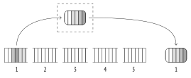
Subsequent rows are then read into the freed memory, and this procedure is repeated until all the data is written into several pre-sorted files.
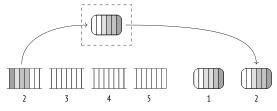
Next, these files are merged into one. This operation is performed by roughly the same algorithm that is used for merge joins; the main difference is that it can process more than two files at a time.
A merge operation does not need too much memory. In fact, it is enough to have room for one row per file. The first rows are read from each file, the row with the lowest value (or the highest one, depending on the sort order) is returned as a partial result, and the freed memory is filled with the next row fetched from the same file.
In practice, rows are read in batches of 32 pages rather than one by one, which reduces the number of I/O operations. The number of files that are merged in a single iteration depends on the available memory, but it is never smaller than six. The upper boundary is also limited (by 500) since efficiency suffers when there are too many files.16
Sorting algorithms have long-established terminology. External sorting was originally performed using magnetic tapes, and PostgreSQL keeps a similar name for the component that controls temporary files.17 Partially sorted data sets are called “runs.”18 The number of runs participating in the merge is referred to as the “merge order.” I did not use these terms, but they are worth knowing if you want to understand PostgreSQL code and comments.
If the sorted temporary files cannot be merged all at once, they have to be processed in several passes, their partial results being written into new temporary files. Each iteration increases the volume of data to be read and written, so the more RAM is available, the faster the external sorting completes.
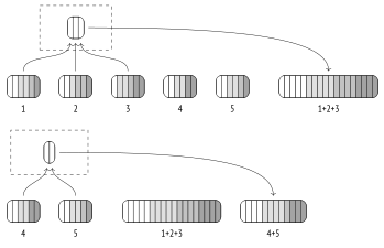
The next iteration merges newly created temporary files.
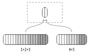
The final merge is typically deferred and performed on the fly when the upper node pulls the data.
Let’s run the EXPLAIN ANALYZE command to see how much disk space has been used by external sorting. The BUFFERS option displays buffer usage statistics for temporary files (temp read and written). The number of written buffers will be (roughly) the same as the number of read ones; converted to kilobytes, this value is shown as Disk in the plan:
To print more details on using temporary files into the server log, you can enable the log_temp_files parameter.
Cost estimation. Let’s take the same plan with external sorting as an example:
Here the regular cost of comparisons (their number is the same as in the case of a quicksort operation in memory) is extended by the I/O cost.19 All the input data has to be first written into temporary files on disk and then read from disk during the merge operation (possibly more than once if all the created files cannot be merged in one iteration).
It is assumed that three quarters of disk operations (both reads and writes) are sequential, while one quarter is random.
The volume of data written to disk depends on the number of rows to be sorted and the number of columns used in the query.20 In this example, the query displays all the columns of the flights table, so the size of the data spilled to disk is almost the same as the size of the whole table if its tuple and page metadata are not taken into account (2309 pages instead of 2624).
Here sorting is completed in one iteration.
Therefore, the sorting cost is estimated in this plan as follows:
Incremental Sorting
If a data set has to be sorted by keys K1 … Km … Kn, and this data set is known to be already sorted by the first m keys, you do not have to re-sort it from scratch. Instead, you can split this set into groups by the same first keys K1 … Km (values in these groups already follow the defined order), and then sort each of these groups separately by the remaining Km+1 … Kn keys. This method is called the incremental sort. (v. 13)
Incremental sorting is less memory-intensive than other sorting algorithms, as it splits the set into several smaller groups; besides, it allows the executor to start returning results after the first group is processed, without waiting for the whole set to be sorted.
In PostgreSQL, the implementation is a bit more subtle:21 while relatively big groups of rows are processed separately, smaller groups are combined together and are sorted in full. It reduces the overhead incurred by invoking the sorting procedure.22
The execution plan represents incremental sorting by the Incremental Sort node:
As the plan shows, the data set is pre-sorted by the total_amount field, as it is the result of an index scan run on this column (Presorted Key). The EXPLAIN ANALYZE command also displays run-time statistics. The Full-sort Groups row is related to small groups that were united to be sorted in full, while the Presorted Groups row displays the data on large groups with partially ordered data, which required incremental sorting by the book_date column only. In both cases, the in-memory quicksort method was applied. The difference in group sizes is due to non-uniform distribution of booking costs.
Incremental sorting can be used to compute window functions too: (v. 14)
Cost estimation. Cost calculations for incremental sorting23 are based on the expected number of groups24 and the estimated sorting cost of an average-sized group (which we have already reviewed).
The startup cost reflects the cost estimation of sorting the first group, which allows the node to start returning sorted rows; the total cost includes the sorting cost of all groups.
We are not going to explore these calculations any further here.
Parallel Mode
Sorting can also be performed concurrently. But although parallel workers do presort their data shares, the Gather node knows nothing about their sort order and can only accumulate them on a first-come, first-serve basis. To preserve the sort order, the executor has to apply the Gather Merge node.25 (v. 10)
The Gather Merge node uses a binary heap26 to adjust the order of rows fetched by several workers. It virtually merges several sorted sets of rows, just like external sorting would do, but is designed for a different use case: Gather Merge typically handles a small fixed number of data sources and fetches rows one by one rather than block by block.
Cost estimation. The startup cost of the Gather Merge node is based on the startup cost of its child node. Just like for the Gather node, this value is increased by the cost of launching parallel processes (estimated at parallel_setup_cost). (p. 303) (default: 1000)
The received value is then further extended by the cost of building a binary heap, which requires sorting n values, where n is the number of parallel workers (that is, n log2 n).
A single comparison operation is estimated at doubled cpu_operator_cost, and total share of such operations is typically negligible since n is quite small. (default: 0.0025)
The total cost includes the expenses incurred by fetching all the data by several processes that perform the parallel part of the plan, and the cost of transferring this data to the leader. A single row transfer is estimated at parallel_tuple_cost increased by 5 %, to compensate for possible waits on getting the next values. (default: 0.1)
The expenses incurred by binary heap updates must also be taken into account in total cost calculations: each input row requires log2 n comparison operations and certain additional actions (they are estimated at cpu_operator_cost).27
Let’s take a look at yet another plan that uses the Gather Merge node. Note that the workers here first perform partial aggregation by hashing, and then the Sort node sorts the received results (it is cheap because few rows are left after aggregation) to be passed further to the leader process, which gathers the full result in the Gather Merge node. As for the final aggregation, it is performed on the sorted list of values: (p. 384)
Here we have three parallel processes (including the leader), and the cost of the Gather Merge node is calculated as follows:
23.3 Distinct Values and Grouping
As we have just seen, grouping values to perform aggregation (and to eliminate duplicates) can be performed not only by hashing, but also by sorting. In a sorted list, groups of duplicate values can be singled out in one pass.
Retrieval of distinct values from a sorted list is represented in the plan by a very simple node called Unique28:
Aggregation is performed in the GroupAggregate node:29
In parallel plans, this node is called Partial GroupAggregate, while the node that completes aggregation is called Finalize GroupAggregate.
Both hashing and sorting strategies can be combined in a single node if grouping is performed by several column sets (specified in the GROUPING SETS, CUBE, or ROLLUP clauses). Without getting into rather complex details of this algorithm, I will simply provide an example that performs grouping by three different columns in conditions of scarce memory: (v. 10)
Here is what happens while this query is being executed. The aggregation node, which is shown in the plan as MixedAggregate, receives the data set sorted by the aircraft_code column.
First, this set is scanned, and the values are grouped by the aircraft_code column (Group Key). As the scan progresses, the rows are reordered by the flight_no column (like it is done by a regular Sort node: either via the quicksort method if the memory is sufficient, or using external sorting on disk); at the same time, the executor places these rows into a hash table that uses departure_airport as its key (like it is done by hash aggregation: either in memory, or using temporary files).
At the second stage, the executor scans the data set that has just been sorted by the flight_no column and groups the values by the same column (Sort Key and the nested Group Key node). If the rows had to be grouped by yet another column, they would be resorted again as required.
Finally, the hash table prepared at the first stage is scanned, and the values are grouped by the departure_airport column (Hash Key).
23.4 Comparison of Join Methods
As we have seen, two data sets can be joined using three different methods, and each of them has its own pros and cons.
The nested loop join does not have any prerequisites and can start returning the first rows of the result set right away. It is the only join method that does not have to fully scan the inner set (as long as index access is available for it). These properties make the nested loop algorithm (combined with indexes) an ideal choice for short OLTP queries, which deal with rather small sets of rows.
The weak point of the nested loop becomes apparent as the data volume grows. For a Cartesian product, this algorithm has quadratic complexity—the cost is proportionate to the product of sizes of the data sets being joined. However, the Cartesian product is not so common in practice; for each row of the outer set, the executor typically accesses a certain number of rows of the inner set using an index, and this average number does not depend on the total size of the data set (for example, an average number of tickets in a booking does not change as the number of bookings and bought tickets grows). Thus, the complexity of the nested loop algorithm often shows linear growth rather than quadratic one, even if with a high linear coefficient.
An important distinction of the nested loop algorithm is its universal applicability: it supports all join conditions, whereas other methods can only deal with equi-joins. It allows running queries with any types of conditions (except for the full join, which cannot be used with the nested loop), but you must keep in mind that a non-equi-join of a large data set is highly likely to be performed slower than desired.
A hash join works best on large data sets. If RAM is sufficient, it requires only one pass over two data sets, so its complexity is linear. Combined with sequential table scans, this algorithm is typically used for OLAP queries, which compute the result based on a large volume of data.
However, if the response time is more important than throughput, a hash join is not the best choice: it will not start returning the resulting rows until the whole hash table is built.
The hash join algorithm is only applicable to equi-joins. Another restriction is that the data type of the join key must support hashing (but almost all of them do).
The nested loop join can sometimes beat the hash join, taking advantage of caching the rows of the inner set in the Memoize node (which is also based on a hash table). While the hash join always scans the inner set in full, the nested loop algorithm does not have to, which may result in some cost reduction. (v. 14)
A merge join can perfectly handle both short OLTP queries and long OLAP ones. It has linear complexity (the sets to be joined have to be scanned only once), does not require much memory, and returns the results without any preprocessing; however, the data sets must already have the required sort order. The most cost-effective way to do it is to fetch the data via an index scan. It is a natural choice if the row count is low; for larger data sets, index scans can still be efficient, but only if the heap access is minimal or does not happen at all.
If no suitable indexes are available, the sets have to be sorted, but this operation is memory-intensive, and its complexity is higher than linear: O(n log2 n). In this case, a hash join is almost always cheaper than a merge join—unless the result has to be sorted.
An added bonus of a merge join is the equivalence of the inner and outer sets. The efficiency of both nested loop and hash joins is highly dependent on whether the planner can assign inner and outer sets correctly.
Merge joins are limited to equi-joins. Besides, the data type must have a B-tree operator class.
The following graph illustrates approximate dependencies between the costs of various join methods and the fraction of rows to be joined.
If the selectivity is high, the nested loop join uses index access for both tables; then the planner switches to the full scan of the outer table, which is reflected by the linear part of the graph.
Here the hash join is using a full scan for both tables. The “step” on the graph corresponds to the moment when the hash table fills the whole memory and the batches start getting spilled to disk.
If an index scan is used, the cost of a merge join shows small linear growth. If the work_mem size is big enough, a hash join is usually more efficient, but a merge join beats it when it comes to temporary files.
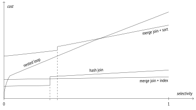
The upper graph of the sort-merge join shows that the costs rise when indexes are unavailable and the data has to be sorted. Just like in the case of a hash join, the “step” on the graph is caused by insufficient memory, as it leads to using temporary files for sorting.
It is merely an example; the ratio between the costs will differ for each particular case.
backend/optimizer/path/joinpath.c, generate_mergejoin_paths function ↩︎
backend/executor/nodeMergejoin.c, ExecMergeJoin function ↩︎
For example, see commitfest.postgresql.org/33/3160 ↩︎
backend/utils/adt/selfuncs.c, mergejoinscansel function ↩︎
backend/optimizer/path/costsize.c, final_cost_mergejoin function ↩︎
backend/optimizer/path/costsize.c, initial_cost_mergejoin & final_cost_mergejoin functions ↩︎
backend/optimizer/path/joinpath.c, consider_parallel_mergejoin function ↩︎
backend/optimizer/path/joinpath.c, select_mergejoin_clauses function ↩︎
backend/optimizer/path/pathkeys.c, build_join_pathkeys function ↩︎
backend/optimizer/path/costsize.c, cost_sort function ↩︎
backend/optimizer/path/costsize.c, cost_sort function ↩︎
backend/utils/sort/tuplesort.c, tuplesort_merge_order function ↩︎
Donald E. Knuth. The Art of Computer Programming. Volume III. Sorting and Searching ↩︎
backend/optimizer/path/costsize.c, cost_sort function ↩︎
backend/optimizer/path/costsize.c, relation_byte_size function ↩︎
backend/optimizer/path/costsize.c, cost_incremental_sort function ↩︎
backend/utils/adt/selfuncs.c, estimate_num_groups function ↩︎
backend/optimizer/path/costsize.c, cost_gather_merge function ↩︎
backend/executor/nodeAgg.c, agg_retrieve_direct function ↩︎