20 Index Scans

PostgreSQL 14 · Translated from Russian by Liudmila Mantrova · Chinese translation by Xiong Cancan

简体中文 · PG14English · PG14简体中文 · PG18 Русский · PG18

20.1 Regular Index Scans

There are two basic ways of accessing TIDs provided by an index. The first one is to perform an index scan. Most of the index access methods (but not all of them) have the INDEX SCAN property to support this operation. (p. 326)

Index scans are represented in the plan by the Index Scan¹ node:

=> EXPLAIN SELECT * FROM bookings
WHERE book_ref = '9AC0C6' AND total_amount = 48500.00;
                 QUERY PLAN
---------------------------------------------
 Index Scan using bookings_pkey on bookings
   (cost=0.43..8.45 rows=1 width=21)
   Index Cond: (book_ref = '9AC0C6'::bpchar)
   Filter: (total_amount = 48500.00)
(4 rows)

During an index scan, the access method returns TIDs one by one.² Upon receiving a TID, the indexing engine accesses the heap page this TID refers to, gets the corresponding tuple, and, if the visibility rules are met, returns the requested set of fields of this tuple. This process continues until the access method runs out of TIDs that matches the query.

The Index Cond line includes only those filter conditions that can be checked using an index. Other conditions that have to be rechecked against the heap are listed separately in the Filter line.

As this example shows, both index and heap access operations are handled by a common Index Scan node rather by two different ones. But there is also a separate Tid Scan node,³ which fetches tuples from the heap if their IDs are known in advance:

=> EXPLAIN SELECT * FROM bookings WHERE ctid = '(0,1)'::tid;
                       QUERY PLAN
---------------------------------------------------------
 Tid Scan on bookings  (cost=0.00..4.01 rows=1 width=21)
   TID Cond: (ctid = '(0,1)'::tid)
(2 rows)

Cost Estimation

Cost estimation of an index scan comprises the estimated costs of index access operations and heap page reads.

Obviously, the index-related part of the estimation fully depends on the particular access method. For B-trees, the cost is mostly incurred by fetching index pages and processing their entries. The number of pages and rows to be read can be determined by the total volume of data and the selectivity of the applied filters. Index pages are accessed at random (pages that follow each other in the logical structure are physically scattered on disk). The estimation is further increased by CPU resources spent on getting from the root to the leaf node and computing all the required expressions.⁴ (p. 262)

The heap-related part of the estimation includes the cost of heap page access and the CPU time required to process all the fetched tuples. It is important to note that I/O estimation depends on both the index scan selectivity and the correlation between the physical order of tuples on disk and the order in which the access method returns their IDs.

Good Scenario: High Correlation

If the physical order of tuples on disk has a perfect correlation with the logical order of TIDs in the index, each page will be accessed only once: the Index Scan node will sequentially go from one page to another, reading the tuples one by one.

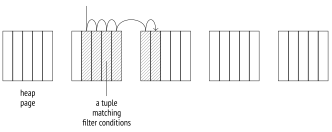
Figure 20.1 Good Scenario: High Correlation

PostgreSQL collects statistics on correlation: (p. 284)

=> SELECT attname, correlation
FROM pg_stats WHERE tablename = 'bookings'
ORDER BY abs(correlation) DESC;
   attname    | correlation
--------------+--------------
 book_ref     |            1
 total_amount | 0.0026738467
 book_date    |  8.02188e-05
(3 rows)

The correlation is high if the corresponding absolute value is close to one (like in the case of book_ref); values that are close to zero are a sign of chaotic data distribution.

Note

In this particular case, high correlation in the book_ref column is of course due to the fact that the data has been loaded into the table in ascending order based on this column, and there have been no updates yet. We would see the same picture if we executed the CLUSTER command for the index created on this column.

However, the perfect correlation does not guarantee that all queries will be returning results in ascending order of book_ref values. First of all, any row update moves the resulting tuple to the end of the table. Second, the plan that relies on an index scan based on some other column returns the results in a different order. And even a sequential scan may not start at the beginning of the table. So if you need a particular order, you should explicitly define it in the ORDER BY clause.

Here is an example of an index scan that processes a large number of rows: (p. 156)

=> EXPLAIN SELECT * FROM bookings WHERE book_ref < '100000';
                 QUERY PLAN
---------------------------------------------
 Index Scan using bookings_pkey on bookings
   (cost=0.43..4638.91 rows=132999 width=21)
   Index Cond: (book_ref < '100000'::bpchar)
(3 rows)

The condition’s selectivity is estimated as follows:

=> SELECT round(132999::numeric/reltuples::numeric, 4)
FROM pg_class WHERE relname = 'bookings';
 round
--------
 0.0630
(1 row)

This value is close to $\frac{1}{16}$ , which we could have guessed knowing that book_ref values range from 000000 to FFFFFF. (p. 280)

For B-trees, the index-related part of the I/O cost estimation includes the cost of reading all the required pages. Index entries that satisfy any condition supported by B-trees are stored in pages bound into an ordered list, so the number of index pages to be read is estimated at the index size multiplied by the selectivity. But since these pages are not physically ordered, reading happens in a random fashion.

CPU resources are spent on processing all the index entries that are read (the cost of processing a single entry is estimated at the cpu_index_tuple_cost value) and computing the condition for each of these entries (in this case, the condition contains a single operator; its cost is estimated at the cpu_operator_cost value). (default: 0.005) (default: 0.0025)

Table access is regarded as sequential reading of the required number of pages. In the case of a perfect correlation, heap tuples will follow each other on disk, so the number of pages is estimated at the size of the table multiplied by the selectivity.

The I/O cost is further extended by the expenses incurred by tuple processing; they are estimated at the cpu_tuple_cost value per tuple. (default: 0.01)

=> WITH costs(idx_cost, tbl_cost) AS (
  SELECT
    (
      SELECT round(
        current_setting('random_page_cost')::real * pages +
        current_setting('cpu_index_tuple_cost')::real * tuples +
        current_setting('cpu_operator_cost')::real * tuples
      )
      FROM (
        SELECT relpages * 0.0630 AS pages, reltuples * 0.0630 AS tuples
        FROM pg_class WHERE relname = 'bookings_pkey'
      ) c
    ),
    (
      SELECT round(
        current_setting('seq_page_cost')::real * pages +
        current_setting('cpu_tuple_cost')::real * tuples
      )
      FROM (
        SELECT relpages * 0.0630 AS pages, reltuples * 0.0630 AS tuples
        FROM pg_class WHERE relname = 'bookings'
      ) c
    )
)
SELECT idx_cost, tbl_cost, idx_cost + tbl_cost AS total
FROM costs;
 idx_cost | tbl_cost | total
----------+----------+-------
     2457 |     2177 |  4634
(1 row)

These calculations illustrate the logic behind the cost estimation, so the result is aligned with the estimation provided by the planner, even if it is approximated. Getting the exact value would require taking other details into account, which we are not going to discuss here.

Bad Scenario: Low Correlation

Everything changes if the correlation is low. Let’s create an index on the book_date column, which has almost zero correlation with this index, and then take a look at the query that selects almost the same fraction of rows as in the previous example. Index access turns out to be so expensive that the planner chooses it only if all the other alternatives are explicitly forbidden:

=> CREATE INDEX ON bookings(book_date);
=> SET enable_seqscan = off;
=> SET enable_bitmapscan = off;
=> EXPLAIN SELECT * FROM bookings
WHERE book_date < '2016-08-23 12:00:00+03';
                             QUERY PLAN
---------------------------------------------------------------------
 Index Scan using bookings_book_date_idx on bookings
   (cost=0.43..56957.48 rows=132403 width=21)
   Index Cond: (book_date < '2016-08-23 12:00:00+03'::timestamp w...
(3 rows)

The thing is that low correlation increases the chances of the next tuple returned by the access method to be located in a different page. Therefore, the Index Scan node has to hop between pages instead of reading them sequentially; in the worst-case scenario, the number of page accesses can reach the number of fetched tuples.

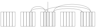
Figure 20.2 Bad Scenario: Low Correlation

However, we cannot simply replace seq_page_cost with random_page_cost and relpages with reltuples in the good-scenario calculations. The cost that we see in the plan is much lower than the value we would have estimated this way:

=> WITH costs(idx_cost, tbl_cost) AS (
  SELECT
    ( SELECT round(
        current_setting('random_page_cost')::real * pages +
        current_setting('cpu_index_tuple_cost')::real * tuples +
        current_setting('cpu_operator_cost')::real * tuples
      )
      FROM (
        SELECT relpages * 0.0630 AS pages, reltuples * 0.0630 AS tuples
        FROM pg_class WHERE relname = 'bookings_pkey'
      ) c
    ),
    ( SELECT round(
        current_setting('random_page_cost')::real * tuples +
        current_setting('cpu_tuple_cost')::real * tuples
      )
      FROM (
        SELECT relpages * 0.0630 AS pages, reltuples * 0.0630 AS tuples
        FROM pg_class WHERE relname = 'bookings'
      ) c
    )
)
SELECT idx_cost, tbl_cost, idx_cost + tbl_cost AS total FROM costs;
 idx_cost | tbl_cost | total
----------+----------+--------
     2457 |   533330 | 535787
(1 row)

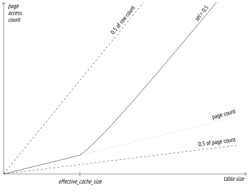
The reason is that the model takes caching into account. Frequently used pages are kept in the buffer cache (and in the OS cache), so the bigger the cache size, the more chances to find the required page in it, thus avoiding an extra disk access operation. For planning purposes, the cache size is defined by the effective_cache_size parameter. The smaller its value, the more pages are expected to be read. (default: 4GB)

The graph that follows shows the dependency between the estimation of the number of pages to be read and the table size (for the selectivity of $\frac{1}{2}$ and the page containing 10 rows).⁵ The dashed lines show the access count in the best scenario possible (half of the page count if the correlation is perfect) and in the worst scenario (half of the row count if there is zero correlation and no cache).

It is assumed that the effective_cache_size value indicates the total volume of memory that can be used for caching (including both the PostgreSQL buffer cache and OS cache). But since this parameter is used solely for estimation purposes and does not affect memory allocation itself, you do not have to take actual figures into account when changing this setting.

$Bad Scenario: Low Correlation: page; countsel = 0.5; 0.5 of row count; access; page count; 0.5 of page count; table size; effective\_cache\_size$

Figure 20.3 Bad Scenario: Low Correlation

If you reduce effective_cache_size to the minimum, the plan estimation will be close to the low-end value shown above for the no-caching case:

=> SET effective_cache_size = '8kB';
=> EXPLAIN SELECT * FROM bookings
WHERE book_date < '2016-08-23 12:00:00+03';
                             QUERY PLAN
---------------------------------------------------------------------
 Index Scan using bookings_book_date_idx on bookings
   (cost=0.43..532745.48 rows=132403 width=21)
   Index Cond: (book_date < '2016-08-23 12:00:00+03'::timestamp w...
(3 rows)
=> RESET effective_cache_size;
=> RESET enable_seqscan;
=> RESET enable_bitmapscan;

The planner calculates the table I/O cost for both worst-case and best-case scenarios and then takes an intermediate value based on the actual correlation.⁶

Thus, an index scan can be a good choice if only a fraction of rows has to be read. If heap tuples are correlated with the order in which the access method returns their IDs, this fraction can be quite substantial. However, if the correlation is low, index scanning becomes much less attractive for queries with low selectivity.

20.2 Index-Only Scans

If an index contains all the heap data required by the query, it is called a covering index for this particular query. If such an index is available, extra table access can be avoided: instead of TIDs, the access method can return the actual data directly. Such a type of an index scan is called an index-only scan.⁷ It can be used by those access methods that support the RETURNABLE property. (p. 328)

In the plan, this operation is represented by the Index Only Scan⁸ node:

=> EXPLAIN SELECT book_ref FROM bookings
WHERE book_ref < '100000';
                   QUERY PLAN
-------------------------------------------------
 Index Only Scan using bookings_pkey on bookings
   (cost=0.43..3791.91 rows=132999 width=7)
   Index Cond: (book_ref < '100000'::bpchar)
(3 rows)

The name suggests that this node never has to access the heap, but it is not so. In PostgreSQL, indexes contain no information on tuple visibility, so the access method returns the data of all the heap tuples that satisfy the filter condition, even if the current transaction cannot see them. Their visibility is then checked by the indexing engine. (p. 74)

However, if this method had to access the table to check visibility of each tuple, it would not be any different from a regular index scan. Instead, it employs the visibility map provided for tables, in which the vacuum process marks the pages that contain only all-visible tuples (that is, those tuples that are accessible to all transactions, regardless of the snapshot used). If the TID returned by the index access method belongs to such a page, there is no need to check its visibility. (p. 27)

The cost estimation of an index-only scan depends on the fraction of all-visible pages in the heap. PostgreSQL collects such statistics:

=> SELECT relpages, relallvisible
FROM pg_class WHERE relname = 'bookings';
 relpages | relallvisible
----------+---------------
    13447 |         13446
(1 row)

The cost estimation of an index-only scan differs from that of a regular index scan: its I/O cost related to table access is taken in proportion to the fraction of pages that do not appear in the visibility map. (The cost estimation of tuple processing is the same.)

Since in this particular example all pages contain only all-visible tuples, the cost of heap I/O is in fact excluded from the cost estimation:

=> WITH costs(idx_cost, tbl_cost) AS (
  SELECT
    (
      SELECT round(
        current_setting('random_page_cost')::real * pages +
        current_setting('cpu_index_tuple_cost')::real * tuples +
        current_setting('cpu_operator_cost')::real * tuples
      )
      FROM (
        SELECT relpages * 0.0630 AS pages,
              reltuples * 0.0630 AS tuples
        FROM pg_class WHERE relname = 'bookings_pkey'
      ) c
    ) AS idx_cost,
    (
      SELECT round(
        (1 - frac_visible) * -- fraction of non-all-visible pages
        current_setting('seq_page_cost')::real * pages +
        current_setting('cpu_tuple_cost')::real * tuples
      )
      FROM (
        SELECT relpages * 0.0630 AS pages,
              reltuples * 0.0630 AS tuples,
          relallvisible::real/relpages::real AS frac_visible
        FROM pg_class WHERE relname = 'bookings'
      ) c
    ) AS tbl_cost
)
SELECT idx_cost, tbl_cost, idx_cost + tbl_cost AS total
FROM costs;
 idx_cost | tbl_cost | total
----------+----------+-------
     2457 |     1330 |  3787
(1 row)

Any unvacuumed changes that have not disappeared behind the database horizon yet increase the estimated cost of the plan (and, consequently, make this plan less attractive to the optimizer). The EXPLAIN ANALYZE command can show the actual heap access count. (p. 88)

In a newly created table, PostgreSQL has to check visibility of all the tuples:

=> CREATE TEMP TABLE bookings_tmp WITH (autovacuum_enabled = off) AS
  SELECT * FROM bookings
  ORDER BY book_ref;
=> ALTER TABLE bookings_tmp ADD PRIMARY KEY(book_ref);
=> ANALYZE bookings_tmp;
=> EXPLAIN (analyze, timing off, summary off)
SELECT book_ref FROM bookings_tmp WHERE book_ref < '100000';
                             QUERY PLAN
---------------------------------------------------------------------
 Index Only Scan using bookings_tmp_pkey on bookings_tmp
   (cost=0.43..4638.91 rows=132999 width=7) (actual rows=132109 l...
   Index Cond: (book_ref < '100000'::bpchar)
   Heap Fetches: 132109
(4 rows)

But once the table has been vacuumed, such a check becomes redundant and is not performed as long as all the pages remain all-visible.

=> VACUUM bookings_tmp;
=> EXPLAIN (analyze, timing off, summary off)
SELECT book_ref FROM bookings_tmp WHERE book_ref < '100000';
                             QUERY PLAN
---------------------------------------------------------------------
 Index Only Scan using bookings_tmp_pkey on bookings_tmp
   (cost=0.43..3787.91 rows=132999 width=7) (actual rows=132109 l...
   Index Cond: (book_ref < '100000'::bpchar)
   Heap Fetches: 0
(4 rows)

Indexes with the Include Clause

It is not always possible to extend an index with all the columns required by a query:

For a unique index, adding a new column would compromise the uniqueness of the original key columns.
The index access method may not provide an operator class for the data type of the column to be added.

In this case, you can still include columns into an index without making them a part of the index key. It will of course be impossible to perform an index scan based on the included columns, but if a query references these columns, the index will function as a covering one. (v. 11)

The following example shows how to replace an automatically created primary key index by another index with an included column:

=> CREATE UNIQUE INDEX ON bookings(book_ref) INCLUDE (book_date);
=> BEGIN;
=> ALTER TABLE bookings
  DROP CONSTRAINT bookings_pkey CASCADE;
NOTICE:  drop cascades to constraint tickets_book_ref_fkey on table
tickets
ALTER TABLE
=> ALTER TABLE bookings ADD CONSTRAINT bookings_pkey PRIMARY KEY
  USING INDEX bookings_book_ref_book_date_idx; -- a new index
NOTICE:  ALTER TABLE / ADD CONSTRAINT USING INDEX will rename index
"bookings_book_ref_book_date_idx" to "bookings_pkey"
ALTER TABLE
=> ALTER TABLE tickets
  ADD FOREIGN KEY (book_ref) REFERENCES bookings(book_ref);
=> COMMIT;

=> EXPLAIN SELECT book_ref, book_date
FROM bookings WHERE book_ref < '100000';
                             QUERY PLAN
---------------------------------------------------------------------
 Index Only Scan using bookings_pkey on bookings  (cost=0.43..437...
   Index Cond: (book_ref < '100000'::bpchar)
(2 rows)

Note

Such indexes are often called covering, but it is not quite correct. An index is considered covering if the set of its columns covers all the columns required by a particular query. It does not matter whether it involves any columns added by the INCLUDE clause, or only key columns are being used. Moreover, an index can be covering for one query but not for the other.

20.3 Bitmap Scans

The efficiency of an index scan is limited: as the correlation decreases, the number of accesses to heap pages rises, and scanning becomes random rather than sequential. To overcome this limitation, PostgreSQL can fetch all the TIDs before accessing the table and sort them in ascending order based on their page numbers.⁹ This is exactly how bitmap scanning works, which is yet another common approach to processing TIDs. It can be used by those access methods that support the BITMAP SCAN property. (p. 326)

Unlike a regular index scan, this operation is represented in the query plan by two nodes:

=> CREATE INDEX ON bookings(total_amount);
=> EXPLAIN SELECT *
FROM bookings WHERE total_amount = 48500.00;
                             QUERY PLAN
---------------------------------------------------------------------
 Bitmap Heap Scan on bookings  (cost=54.63..7040.42 rows=2865 wid...
   Recheck Cond: (total_amount = 48500.00)
   -> Bitmap Index Scan on bookings_total_amount_idx
       (cost=0.00..53.92 rows=2865 width=0)
       Index Cond: (total_amount = 48500.00)
(5 rows)

The Bitmap Index Scan¹⁰ node gets the bitmap of all TIDs¹¹ from the access method.

The bitmap consists of separate segments, each corresponding to a single heap page. All these segments have the same size, which is enough for all the page tuples, no matter how many of them are present. This number is limited because a tuple header is quite large; a standard-size page can accommodate 256 tuples at the most, which fit 32 bytes.¹²

Then the Bitmap Heap Scan¹³ traverses the bitmap segment by segment, reads the corresponding pages, and checks all their tuples that are marked all-visible. Thus, pages are read in ascending order based on their numbers, and each of them is read exactly once.

That said, this process is not the same as sequential scanning since the accessed pages rarely follow each other. Regular prefetching performed by the operating system does not help in this case, so the Bitmap Heap Scan node implements its own prefetching by asynchronously reading effective_io_concurrency pages—and it is the only node that does it. This mechanism relies on the posix_fadvise function implemented by some operating systems. If your system happens to support this function, it makes sense to configure the effective_io_concurrency parameter at the tablespace level in accordance with the hardware capabilities. (default: 1)

Note

Asynchronous prefetching is also used by some other internal processes:

for index pages when heap rows are being deleted¹⁴ (v. 13)
for heap pages during analysis (ANALYZE)¹⁵ (v. 14) (default: 10)

Note

The prefetch depth is defined by the maintenance_io_concurrency.

Bitmap Accuracy

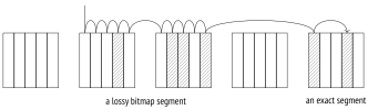
The more pages contain the tuples that satisfy the filter condition of the query, the bigger is the bitmap. It is built in the local memory of the backend, and its size is limited by the work_mem parameter. Once the maximum allowed size is reached, some bitmap segments become lossy: each bit of a lossy segment corresponds to a whole page, while the segment itself comprises a range of pages.¹⁶ As a result, the size of the bitmap becomes smaller at the expense of its accuracy. (default: 4MB)

The EXPLAIN ANALYZE command shows the accuracy of the built bitmap:

=> EXPLAIN (analyze, costs off, timing off, summary off)
SELECT * FROM bookings WHERE total_amount > 150000.00;
                             QUERY PLAN
---------------------------------------------------------------------
 Bitmap Heap Scan on bookings (actual rows=242691 loops=1)
   Recheck Cond: (total_amount > 150000.00)
   Heap Blocks: exact=13447
   -> Bitmap Index Scan on bookings_total_amount_idx (actual rows...
       Index Cond: (total_amount > 150000.00)
(5 rows)

Here we have enough memory for an exact bitmap.

If we decrease the work_mem value, some of the bitmap segments become lossy:

=> SET work_mem = '512kB';
=> EXPLAIN (analyze, costs off, timing off, summary off)
SELECT * FROM bookings WHERE total_amount > 150000.00;
                             QUERY PLAN
---------------------------------------------------------------------
 Bitmap Heap Scan on bookings (actual rows=242691 loops=1)
   Recheck Cond: (total_amount > 150000.00)
   Rows Removed by Index Recheck: 1145721
   Heap Blocks: exact=5178 lossy=8269
   -> Bitmap Index Scan on bookings_total_amount_idx (actual rows...
       Index Cond: (total_amount > 150000.00)
(6 rows)
=> RESET work_mem;

When reading a heap page that corresponds to a lossy bitmap segment, PostgreSQL has to recheck the filter condition for each tuple in the page. The condition to be rechecked is always displayed in the plan as Recheck Cond, even if this recheck is not performed. The number of tuples filtered out during a recheck is displayed separately (as Rows Removed by Index Recheck).

Note

If the size of the result set is too big, the bitmap may not fit the work_mem memory chunk, even if all its segments are lossy. Then this limit is ignored, and the bitmap takes as much space as required. PostgreSQL neither further reduces the bitmap accuracy nor flushes any of its segments to disk.

Operations on Bitmaps

If the query applies conditions to several table columns that have separate indexes created on them, a bitmap scan can use several indexes together.¹⁷ All these indexes have their own bitmaps built on the fly; the bitmaps are then combined together bit by bit, using either logical conjunction (if the expressions are connected by AND) or logical disjunction (if the expressions are connected by OR). For example:

=> EXPLAIN (costs off)
SELECT * FROM bookings
WHERE book_date < '2016-08-28'
  AND total_amount > 250000;
                             QUERY PLAN
---------------------------------------------------------------------
 Bitmap Heap Scan on bookings
   Recheck Cond: ((total_amount > '250000'::numeric) AND (book_da...
   -> BitmapAnd
       -> Bitmap Index Scan on bookings_total_amount_idx
           Index Cond: (total_amount > '250000'::numeric)
       -> Bitmap Index Scan on bookings_book_date_idx
           Index Cond: (book_date < '2016-08-28 00:00:00+03'::tim...
(7 rows)

Here the BitmapAnd node combines two bitmaps using the bitwise AND operation.

As two bitmaps are being merged into one,¹⁸ exact segments remain exact when merged together (if the new bitmap fits the work_mem memory chunk), but if any segment in a pair is lossy, the resulting segment will be lossy too.

Cost Estimation

Let’s take a look at the query that uses a bitmap scan:

=> EXPLAIN
SELECT * FROM bookings
WHERE total_amount = 28000.00;
                             QUERY PLAN
---------------------------------------------------------------------
 Bitmap Heap Scan on bookings  (cost=599.48..14444.96 rows=31878 ...
   Recheck Cond: (total_amount = 28000.00)
   -> Bitmap Index Scan on bookings_total_amount_idx
       (cost=0.00..591.51 rows=31878 width=0)
       Index Cond: (total_amount = 28000.00)
(5 rows)

The approximate selectivity of the condition used by the planner equals

=> SELECT round(31878::numeric/reltuples::numeric, 4)
FROM pg_class WHERE relname = 'bookings';
 round
--------
 0.0151
(1 row)

The total cost of the Bitmap Index Scan node is estimated in the same way as the cost of a regular index scan that does not take heap access into account:

=> SELECT round(
  current_setting('random_page_cost')::real * pages +
  current_setting('cpu_index_tuple_cost')::real * tuples +
  current_setting('cpu_operator_cost')::real * tuples
)
FROM (
  SELECT relpages * 0.0151 AS pages, reltuples * 0.0151 AS tuples
  FROM pg_class WHERE relname = 'bookings_total_amount_idx'
) c;
 round
-------
   589
(1 row)

The I/O cost estimation for the Bitmap Heap Scan node differs from that for a perfect-correlation case of a regular index scan. A bitmap allows reading heap pages in ascending order based on their numbers, without getting back to the same page, but the tuples that satisfy the filter condition do not follow each other anymore. Instead of reading a strictly sequential page range that is quite compact, PostgreSQL is likely to access far more pages.

Figure 20.4 Cost Estimation

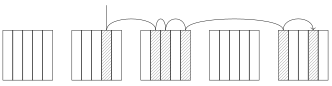
The number of pages to be read is estimated by the following formula:¹⁹

\min\!\left(\frac{2\,\mathtt{relpages}\cdot\mathtt{reltuples}\cdot\mathtt{sel}}{2\,\mathtt{relpages}+\mathtt{reltuples}\cdot\mathtt{sel}},\ \mathtt{relpages}\right)

The estimated cost of reading a single page falls between seq_page_cost and random_page_cost, depending on the ratio of the fraction of fetched pages to the total number of pages in the table:

=> WITH t AS (
  SELECT relpages,
    least(
      (2 * relpages * reltuples * 0.0151) /
      (2 * relpages + reltuples * 0.0151),
      relpages
    ) AS pages_fetched,
    round(reltuples * 0.0151) AS tuples_fetched,
    current_setting('random_page_cost')::real AS rnd_cost,
    current_setting('seq_page_cost')::real AS seq_cost
  FROM pg_class WHERE relname = 'bookings'
)
SELECT pages_fetched,
  rnd_cost - (rnd_cost - seq_cost) *
  sqrt(pages_fetched / relpages) AS cost_per_page,
  tuples_fetched
FROM t;
 pages_fetched | cost_per_page | tuples_fetched
---------------+---------------+----------------
         13447 |             1 |          31878
(1 row)

As usual, the I/O estimation is increased by the cost of processing each fetched tuple. If an exact bitmap is used, the number of tuples is estimated at the total number of tuples in the table multiplied by the selectivity of filter conditions. But if any bitmap segments are lossy, PostgreSQL has to access the corresponding pages to recheck all their tuples.

Figure 20.5 Cost Estimation

Thus, the estimation takes into account the expected fraction of lossy bitmap segments (which can be calculated based on the total number of selected rows and the bitmap size limit defined by work_mem).²⁰ (v. 11)

The total cost of condition rechecks also increases the estimation (regardless of the bitmap accuracy).

The startup cost estimation of the Bitmap Heap Scan node is based on the total cost of the Bitmap Index Scan node, which is extended by the cost of bitmap processing:

                     QUERY PLAN
-----------------------------------------------------
 Bitmap Heap Scan on bookings
   (cost=599.48..14444.96 rows=31878 width=21)
   Recheck Cond: (total_amount = 28000.00)
   -> Bitmap Index Scan on bookings_total_amount_idx
       (cost=0.00..591.51 rows=31878 width=0)
       Index Cond: (total_amount = 28000.00)
(6 rows)

Here the bitmap is exact, and the cost is estimated roughly as follows:²¹

=> WITH t AS (
  SELECT 1 AS cost_per_page,
         13447 AS pages_fetched,
         31878 AS tuples_fetched
),
costs(startup_cost, run_cost) AS (
  SELECT
    ( SELECT round(
        589 /* cost estimation for the child node */ +
        0.1 * current_setting('cpu_operator_cost')::real *
        reltuples * 0.0151
      )
      FROM pg_class WHERE relname = 'bookings_total_amount_idx'
    ),
    ( SELECT round(
        cost_per_page * pages_fetched +
        current_setting('cpu_tuple_cost')::real * tuples_fetched +
        current_setting('cpu_operator_cost')::real * tuples_fetched
      )
      FROM t
    )
)
SELECT startup_cost, run_cost,
  startup_cost + run_cost AS total_cost
FROM costs;
 startup_cost | run_cost | total_cost
--------------+----------+------------
          597 |    13845 |      14442
(1 row)

If the query plan combines several bitmaps, the sum of the costs of separate index scans is increased by a (small) cost of merging them together.²²

20.4 Parallel Index Scans

All the index scanning modes—a regular index scan, an index-only scan, and a bitmap scan—have their own flavors for parallel plans. (v. 9.6) (p. 300)

The cost of parallel execution is estimated in the same way as that of sequential one, but (just like in the case of a parallel sequential scan) CPU resources are distributed between all parallel processes, thus reducing the total cost. The I/O component of the cost is not distributed because processes are synchronized to perform page access sequentially.

Now let me show you several examples of parallel plans without breaking down their cost estimation.

A parallel index scan:

=> EXPLAIN SELECT sum(total_amount)
FROM bookings WHERE book_ref < '400000';
                             QUERY PLAN
---------------------------------------------------------------------
 Finalize Aggregate  (cost=19192.81..19192.82 rows=1 width=32)
   -> Gather  (cost=19192.59..19192.80 rows=2 width=32)
       Workers Planned: 2
       -> Partial Aggregate  (cost=18192.59..18192.60 rows=1 widt...
           -> Parallel Index Scan using bookings_pkey on bookings
               (cost=0.43..17642.82 rows=219907 width=6)
               Index Cond: (book_ref < '400000'::bpchar)
(7 rows)

While a parallel scan of a B-tree is in progress, the ID of the current index page is kept in the server’s shared memory. The initial value is set by the process that starts the scan: it traverses the tree from the root to the first suitable leaf page and saves its ID. Workers access subsequent index pages as needed, replacing the saved ID. Having fetched a page, the worker iterates through all its suitable entries and reads the corresponding heap tuples. The scanning completes when the worker has read the whole range of values that satisfy the query filter.

A parallel index-only scan:

=> EXPLAIN SELECT sum(total_amount)
FROM bookings WHERE total_amount < 50000.00;
                             QUERY PLAN
---------------------------------------------------------------------
 Finalize Aggregate  (cost=23370.60..23370.61 rows=1 width=32)
   -> Gather  (cost=23370.38..23370.59 rows=2 width=32)
       Workers Planned: 2
       -> Partial Aggregate  (cost=22370.38..22370.39 rows=1 widt...
           -> Parallel Index Only Scan using bookings_total_amoun...
               (cost=0.43..21387.27 rows=393244 width=6)
               Index Cond: (total_amount < 50000.00)
(7 rows)

A parallel index-only scan skips heap access for all-visible pages; it is the only difference it has from a parallel index scan.

A parallel bitmap scan:

=> EXPLAIN SELECT sum(total_amount)
FROM bookings WHERE book_date < '2016-10-01';
                             QUERY PLAN
---------------------------------------------------------------------
 Finalize Aggregate  (cost=21492.21..21492.22 rows=1 width=32)
   -> Gather  (cost=21491.99..21492.20 rows=2 width=32)
       Workers Planned: 2
       -> Partial Aggregate  (cost=20491.99..20492.00 rows=1 widt...
           -> Parallel Bitmap Heap Scan on bookings
               (cost=4891.17..20133.01 rows=143588 width=6)
               Recheck Cond: (book_date < '2016-10-01 00:00:00+03...
               -> Bitmap Index Scan on bookings_book_date_idx
                   (cost=0.00..4805.01 rows=344611 width=0)
                   Index Cond: (book_date < '2016-10-01 00:00:00+...
(10 rows)

A bitmap scan implies that a bitmap is always built sequentially, by a single leader process; for this reason, the name of the Bitmap Index Scan node does not contain the word Parallel. When the bitmap is ready, the Parallel Bitmap Heap Scan node starts a parallel heap scan. Workers access subsequent heap pages and process them concurrently.

20.5 Comparison of Various Access Methods

The following illustration shows how costs of various access methods depend on selectivity of filter conditions:

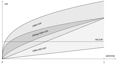
Figure 20.6 20.5 Comparison of Various Access Methods

It is a qualitative diagram; the actual figures are of course dependent on the particular table and server configuration.

Sequential scanning does not depend on selectivity, and starting from a certain fraction of selected rows, it is usually more efficient than other methods.

The cost of an index scan is affected by the correlation between the physical order of tuples and the order in which their IDs are returned by the access method. If the correlation is perfect, an index scan can be quite efficient even if the fraction of selected rows is rather high. However, for low correlation (which is much more common) it can quickly become even more expensive than a sequential scan. That said, index scanning is still an absolute leader when it comes to selecting a single row using an index (typically a unique one).

If applicable, index-only scans can show great performance and beat sequential scans even if all the rows are selected. However, their performance is highly dependent on the visibility map, and in the worst-case scenario an index-only scan can degrade to a regular index scan.

The cost of a bitmap scan is affected by the size of available memory, but to a much lesser extent than an index scan cost depends on correlation. If the correlation is low, the bitmap scan turns out to be much cheaper.

Each access method has its own perfect usage scenarios; there is no such method that always outperforms other methods. The planner has to do extensive calculations to estimate the efficiency of each method in each particular case. Clearly, the accuracy of these estimations highly depends on the accuracy of the collected statistics.

backend/executor/nodeIndexscan.c ↩︎
backend/access/index/indexam.c, index_getnext_tid function ↩︎
backend/executor/nodeTidscan.c ↩︎
backend/utils/adt/selfuncs.c, btcostestimate function postgresql.org/docs/14/index-cost-estimation.html ↩︎
backend/optimizer/path/costsize.c, index_pages_fetched function ↩︎
backend/optimizer/path/costsize.c, cost_index function ↩︎
postgresql.org/docs/14/indexes-index-only-scans.html ↩︎
backend/executor/nodeIndexonlyscan.c ↩︎
backend/access/index/indexam.c, index_getbitmap function ↩︎
backend/executor/nodeBitmapIndexscan.c ↩︎
backend/access/index/indexam.c, index_getbitmap function ↩︎
backend/nodes/tidbitmap.c ↩︎
backend/executor/nodeBitmapHeapscan.c ↩︎
backend/access/heap/heapam.c, index_delete_prefetch_buffer function ↩︎
backend/commands/analyze.c, acquire_sample_rows function ↩︎
backend/nodes/tidbitmap.c, tbm_lossify function ↩︎
postgresql.org/docs/14/indexes-ordering.html ↩︎
backend/nodes/tidbitmap.c, tbm_union & tbm_intersect functions ↩︎
backend/optimizer/path/costsize.c, compute_bitmap_pages function ↩︎
backend/optimizer/path/costsize.c, compute_bitmap_pages function ↩︎
backend/optimizer/path/costsize.c, cost_bitmap_heap_scan function ↩︎
backend/optimizer/path/costsize.c, cost_bitmap_and_node & cost_bitmap_or_node functions ↩︎